
The detection of muons is an important task in the CMS experiment at CERN (European Organization for Nuclear Research). Muons are usually expected to be produced by many physical experiments studied in depth at the CMS physics program at CERN. For example, one way to study the famous Higgs Boson particle is through a decay channel where the Higgs Boson decays into four muons.
Since muons can penetrate several meters of iron with no significant energy loss, they are hardly stopped by any layer of the CMS system. Therefore, the muon detectors are the outermost ones, far from the interaction point. The current muon transverse momentum detector, the Barrel Muon Track Finder, uses Lookup Tables to estimate the transverse momentum of the muons. The latter is measured using the pseudo-rapidity eta, a spatial quantity related to the angle at which the charged particles emerge from these collisions, and the azimuth angle phi, the angle that the collision paths make with the z-axis. (Source: CMS Level-1 Trigger Muon Momentum assignment with Machine Learning - Tommaso Diotalevi)
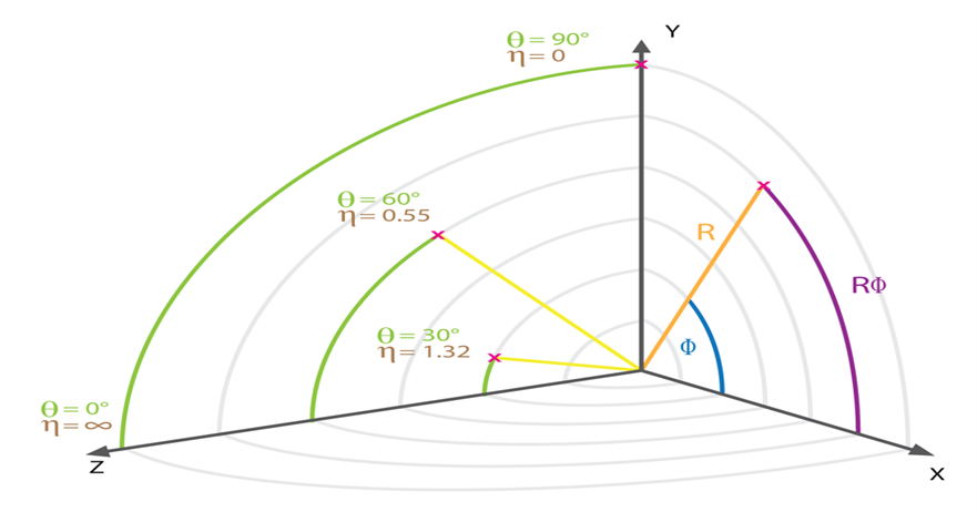
Figure 1: Adopted Coordinate System
Any detection of the muon at this level is called a trigger.
Problem Description
Much more sophisticated techniques are needed to improve the precision of the momentum detection to reduce the trigger rates. Since the prompt muon spectrum follows an exponential distribution, any small improvement in the precision might significantly reduce the number of triggers, especially by reducing the number of low momentum muons misclassified as high momentum muons.
And that’s where machine learning comes into place. By applying smarter algorithms such as Neural Networks, we can improve the precision of the trigger systems to accurately detect the muons and their corresponding transverse momenta. (Source: CMS Level-1 Trigger Muon Momentum assignment with Machine Learning - Tommaso Diotalevi)
In the following article, we will try to use several Deep Learning approaches to accurately predict muon momentum. We will use Monte-Carlo simulated data from the Cathode Strip Chambers (CSC) at the CMS experiment. The dataset contains more than 3 million muon events generated using Pythia.
You can also check the Jupyter notebook we prepared for preprocessing and training the models here.
Exploring the Dataset
The data we retrieved is organized as follows:
There are 87 features: 84 related to the detectors and 3 serving as path variables
There are 12 detector planes inside the CSC and each has 7 features (12*7=84)
The features are organized in the following table:
Column Range 0-11 12-23 24-35 36-47 48-59 60-71 72-83 84-86 features Phi coordinate Theta coordinate Bending angle Time info Ring number Front/rear hit Mask X_road
Table 1: Features and their indices in the dataset
In addition to other features:
| Column Range | 87 | 88 | 89 |
|---|---|---|---|
| features | Phi angle | Eta angle | q/pt (Muon Momentum) - target label |
Table 2: Additional Features and their indices in the dataset
Inside the muon chamber, there are multiple detector stations as it is shown in the figure below. These detector planes are organized in specific chambers. Figure 2: Schematic view of a CMS quadrant (Source: CERN Document Server)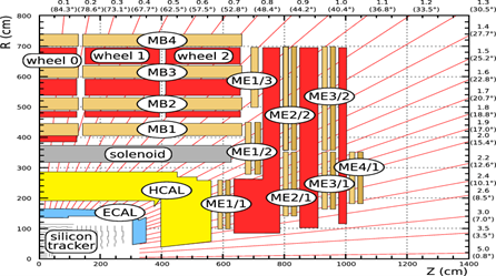
However, we only care about the muon hits in the CSC chambers and therefore features related to the CSC chambers only.
Let us first delete those unneeded features:
Now that we deleted those features, we can next fit all the features into a compact Pandas data frame for easier data analysis later on.
Exploratory Data Analysis
Let’s start by taking a look on the data statistics using Pandas’ describe method:
| Phi angle1 | Theta angle1 | Bend angle1 | Time1 | Ring1 | Front/Rear1 | |
|---|---|---|---|---|---|---|
| count | 870666.0 | 870666.0 | 870666.0 | 870666.0 | 870666.0 | 870666.0 |
| mean | 2942.738281 | 62.888813 | -0.075262 | -0.029150 | 2.0 | 0.465420 |
| std | 1061.839233 | 10.498766 | 19.846676 | 0.167572 | 0.0 | 0.499028 |
| min | 690.000000 | 46.000000 | -81.000000 | -1.000000 | 2.0 | 0.000000 |
| 25% | 2032.000000 | 54.000000 | -14.000000 | 0.000000 | 2.0 | 0.000000 |
| 50% | 2937.000000 | 62.000000 | 0.000000 | 0.000000 | 2.0 | 0.000000 |
| 75% | 3853.000000 | 71.000000 | 14.000000 | 0.000000 | 2.0 | 1.000000 |
| max | 4950.000000 | 88.000000 | 70.000000 | 0.000000 | 2.0 | 1.000000 |
Table 3: Statistics about features with missing values
A quick look reveals that some features such as Phi angle1, Theta angle1 and Bend angle1 have some missing values. Let’s find the exact percentage of null values for each feature:
Figure 3: Missing values distribution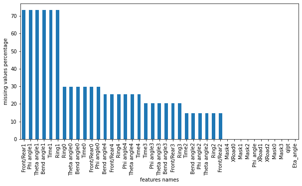
We notice that Front/Rear1, Phi angle1, Theta angle1, Bend angle1, Time1 and Ring1 features have more than 70% missing values! We need to remove those features later on, and for the other features with less than 25% of missing values, we will fill the missing values with each column’s mean.
Next, we will visualize the data distribution of all features.
Figure 4: Selected features histograms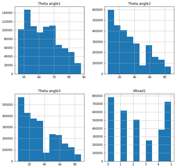
We notice as shown in the figure above that some features such as Theta angle1, Theta angle2, Theta angle3 and X Road1 need to be transformed into Normal distributions (using Standardization) if we want to improve the learning speed of the model.
Data Preprocessing for Training
Framing the Problem as a Classification Task
Instead of trying to apply regression to predict the muon momenta values (q/pt), let’s first try to cluster the momenta into 4 classes: 0-10 GeV, 10-30 GeV, 30-100 GeV and >100 GeV, and hence frame the problem as a classification task.
In order to group the momenta, we will use the absolute value of the reciprocal of the target feature (pt/q). Figure 5: The data distribution of the target feature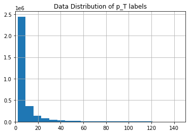
As shown in figure, it is clear that there are distinct groups of different magnitude. We can use the cut method from Pandas to cluster the muon momenta:
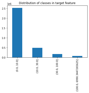
Figure 6: The data distribution of the target classes
Now we have successfully grouped the labels!
We can observe that the classes are not balanced, therefore we need to balance those classes whenever we start training our Neural Network to avoid any bias.
Splitting the Dataset into Train and Test sets
Next, let’s separate the data into train and test data, we will use a 90%-10% split.
It is important to make the test set representative of the target classes distribution in the original dataset. Therefore, instead of randomly splitting our original dataset, we will use the StratifiedShuffleSplit method in Scikit-Learn to make both the train data and test data representative of the original distribution of classes.
Let’s check the classes distribution in the newly generated sets:
| Classes | Original | Train | Test |
|---|---|---|---|
| (0.0, 10.0] | 77.201062 | 77.201058 | 77.201094 |
| (10.0, 30.0] | 15.207951 | 15.207942 | 15.208031 |
| (30.0, 100.0] | 5.331871 | 5.331862 | 5.331948 |
| (100.0, 6990.34] | 2.259117 | 2.259138 | 2.258927 |
Table 4: Comparing the classes distribution between the original, train and test sets
As the previous table shows, both the train set and test set are representative of the original dataset. We can now safely proceed to the final step of preprocessing: preparing the pipeline.
Preparing the Preprocessing Pipeline
This pipeline will perform the following tasks:
Delete columns with missing values more than 70%
Impute the other columns with missing values with their corresponding means using Scikit-Learn Simple Imputer
Standardize the data with Scikit-Learn Standard Scaler
Encode the target feature into four one hot encoded features
Here is the pipeline full code:
Building the Neural Network
We will use Tensorflow’s Keras library to build our Neural Network. The Neural Network will have 5 hidden layers with number of neurons in each layers is 512, 256, 128, 64 and 32. We also added dropout layers to the network to reduce overfitting. The output layer will have 4 neurons (same as the number of classes) and we will apply the softmax activation function to each output neuron to get the probability of each class.
Since it is a classification task, our loss function of choice is the categorical cross entropy. Adam will be used as optimizer.
Let’s set some callbacks for the model including a Checkpoint callback and Early Stopping callback that will both monitor the model’s validation accuracy. We will use a 25% validation split, batch size of 500 and will train for 200 epochs. And now we can finally start training!
Now that we finished training our model, let’s take a look at the evolution of its performance over the training epochs. Figure 7: Evolution of classifier metrics over training epochs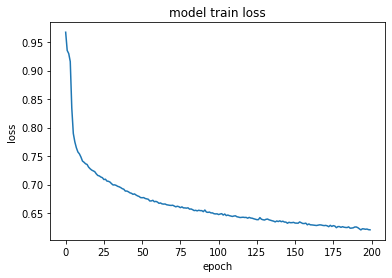
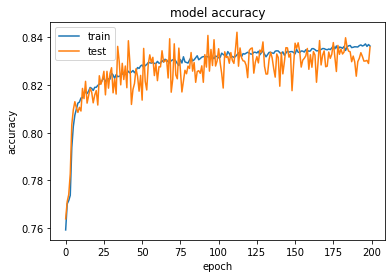
It looks like we achieved an 84% accuracy on the validation set! That’s impressive! But if there is only one thing I have learned by heart from Machine Learning, it will be to never rely on accuracy only to judge the model performance. We need to go deeper to understand the case better.
Testing the Model
Let’s examine the performance of the model on the train set and the test set using Scikit-Learn’s classification report. It includes an array of important classification metrics including precision, recall and f1-score.
| Train Report | Precision | Recall | f1-score |
|---|---|---|---|
| 0 | 0.99 | 0.90 | 0.94 |
| 1 | 0.65 | 0.59 | 0.62 |
| 2 | 0.33 | 0.73 | 0.46 |
| 3 | 0.36 | 0.66 | 0.47 |
| Macro Average | 0.58 | 0.72 | 0.62 |
| Weighted Average | 0.89 | 0.84 | 0.86 |
Table 5: Train data evaluation report
| Test Report | Precision | Recall | f1-score |
|---|---|---|---|
| 0 | 0.99 | 0.90 | 0.94 |
| 1 | 0.64 | 0.58 | 0.61 |
| 2 | 0.32 | 0.70 | 0.44 |
| 3 | 0.33 | 0.61 | 0.43 |
| Macro Average | 0.57 | 0.70 | 0.61 |
| Weighted Average | 0.89 | 0.84 | 0.85 |
Table 6: Test data evaluation report
That’s impressive! It seems that adding class weights definitely reduced bias and we reached a weighted f1-score of 0.85 on the test data!
Experimenting with Regression
Instead of classifying the target label into four group, let us try to directly predict the q/pT value for each muon momentum, therefore framing the problem as a regression task.
We only changed the last layer of the model, and replaced the 4 neurons with softmax by one output neuron with a linear activation function.
Since it is a regression task, we will choose mean square error as our loss function , and similarly to the classification task, we will use Adam as optimizer.
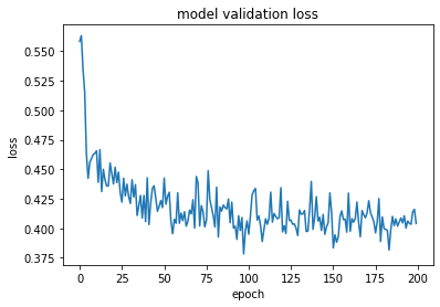
Let’s take a look on the evolution of the regression model’s performance over training epochs: Figure 7: Evolution of the model train and validation loss over training epochs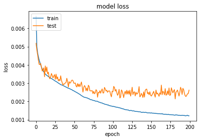
The root mean squared error for the train data is 0.046 and for the test data is 0.047. Not bad at all! The values seems to be relatively acceptable in comparison to the target value, but definitely there is room for improvement.
Future Directions
We discovered that the classifier model was not very good in detecting minority classes. Therefore we need to look for more techniques to make the model less biased (such as up sampling minority classes or down sampling the majority class).
We can further improve the performance of our regression model by hyperparameter tuning through grid search.
Final Thoughts
In this project, we tried several deep learning approaches to accurately predict muon momentum. At first, we investigated the data properties before preprocessing the data for training. We then trained a classifier to predict muon momentum class and evaluated the performance of the classifier on new data using multiple classification metrics. Next, we trained a regression model to predict muon momentum values instead of their classes. Both approaches turned out to be successful, and we plan to incorporate more advanced techniques to reduce model bias and improve its performance.